

Symbol-to-Instrument Neural Generator
Alexandre Défossez1,2,3,4
with Neil Zeghidour1,2,3,4, Nicolas Usunier1, Léon Bottou1 and
Francis Bach2,3,4.
1FAIR / 2École Normale Supérieure
/ 3INRIA / 4PSL Research University
Slides available at https://ai.honu.io
Plan for today
Sound generation with deep learning
Motivation
Vocoder: transforms input parameters into sound. Used for telecommunications, speech and instrument synthesis etc.
Historically hand crafted by signal processing experts.
Deep learning based vocoder: transform high level representation (words, notes etc) into sound, automatically tuned for any application.
Applications: text-to-speech, synthesis of new instruments, style transfer (whistling to symphonic orchestra) etc.
The phase problem
The STFT of a signal is complex valued.
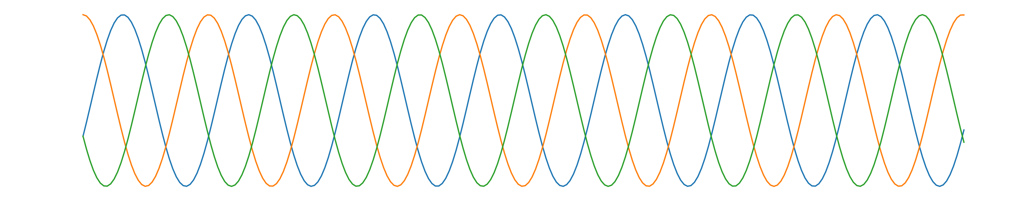
All signals sound the same but different phase values.
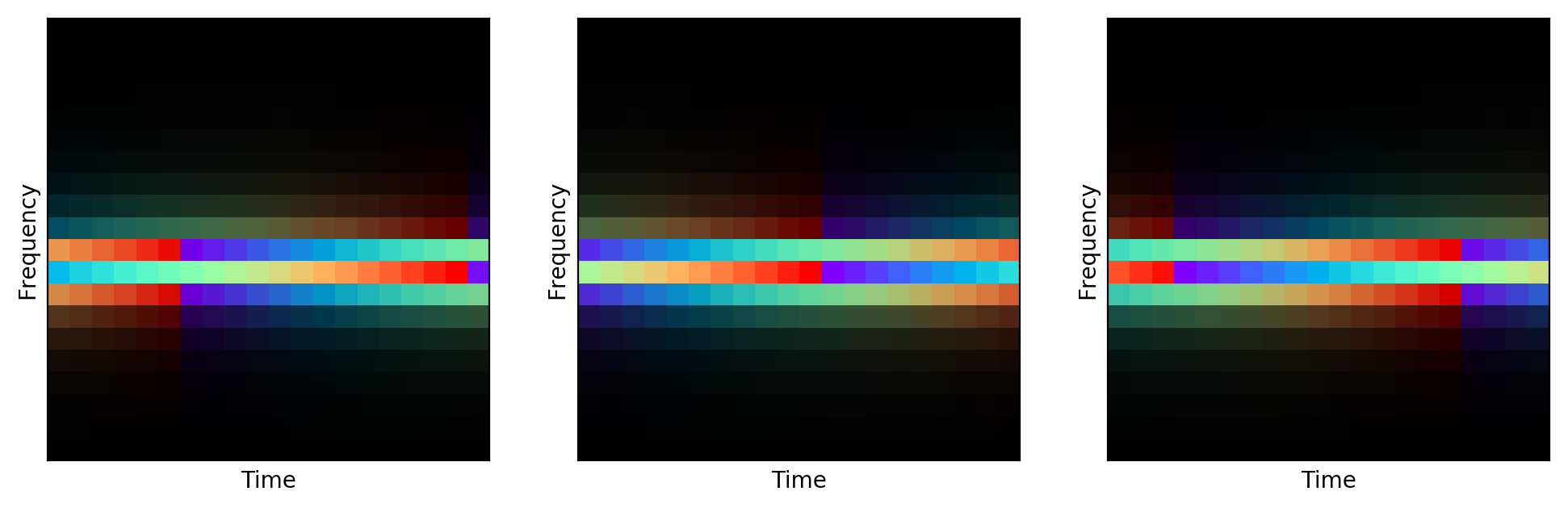
Color is phase and intensity is log power.
The phase problem
Phase is hard. Classification (speech detection) works only on the amplitude.
Phase is necessary for the inverse transform, spectrogram to waveform.
Phase recovery algorithm: Griffin-Lim.
Problem: not all amplitude spectrogram come from a real signal.
Errors in prediction impact final signal in ways that cannot be controled end-to-end.
Tacotron: speech synthesis with Griffin-Lim
At the time, state of the art speech synthesis developed at Google. [Wang et al 2017]
Predicts amplitude spectrogram and inverse with Griffin-Lim.

Direct waveform generation with Wavenet
First succesful approach to direct waveform generation [ Oord et al 2016].
Deep auto-regressive convolutional network that models \[ \mathbb{P}\left[x(t) = y | x(t-1), x(t-2), \ldots, x(t-L)\right] \]
Tacotron 2: speech generation using Wavenet
New state of the art using Wavenet. [Shen et al 2017]
Generates mel-spectrogram and uses Wavenet to generate waveform.
Not quite end-to-end but improved inversion compared to Griffin-Lim.

Tacotron 1:
Tacotron 2:
What's left to explore ?
Wavenet redefined the state of the art.
Cost of training is enormous. On a typical task, can require as much as 32 GPUs for 10 days.
Because it is auto-regressive, evaluation is very slow. Original model is less than real time. Parallel wavenet [Oord et al 2017] solve the problem but requires even longer training.
Little control over the loss with Wavenet.
Plan for today
SING: a lightweight sound generator
NSynth: a music notes dataset
Dataset of 300,000 notes from 1,000 instruments released by the Magenta team at Google [blog].
Each note is 4 seconds sampled at 16kHz, so dimension 64,000. Each note indexed by a unique triplet $(P, I, V)$ (Pitch, Instrument, Velocity).
Goal
Fast training and generation for music note synthesis.
Completion: for each instrument, 10% of the pitches are randomely selected for a test set.
Learn a disantangled representation of the pitch and timbre, i.e. allow changing one without changing the other.
End-to-end loss on the generated waveform.
Reconstruction loss
We want to evaluate the distance between the generated waveform $\hat{x}$ and the ground truth $x$. Either MSE on the waveform: \[ \newcommand{\abs}[1]{\left|#1\right|} \newcommand{\norm}[1]{\left\|#1\right\|} \newcommand{\Lwav}[1]{\mathrm{L}_{\mathrm{wav}}\left(#1\right)} \newcommand{\Lspec}[1]{\mathrm{L}_{\mathrm{stft,1}}\left(#1\right)} \newcommand{\STFT}[1]{\mathrm{STFT}\left[#1\right]} \newcommand{\reel}{\mathbb{R}} \Lwav{x, \hat{x}} := \norm{x - \hat{x}}^2, \]
or using a spectral loss: \[ \Lspec{x, \hat{x}} := \norm{l(x) - l(\hat{x})}_1 \] where $ l(x) := \log\left(1 + \abs{\STFT{x}}^2\right)$.
Model architecture
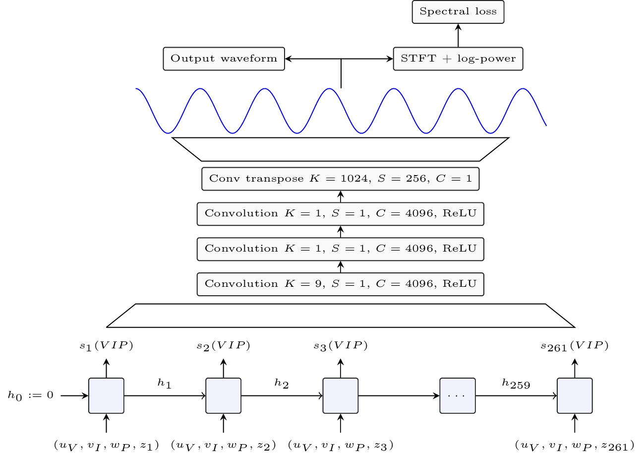
LSTM-based sequence generator output temporal embeddings at $62$ Hz.
Convolutional learnt upsampling turns it into a $16$ kHz waveform.
Sequence generator

Input is learned embedding (a.k.a lookup-table) for the velocity $u_V \in \reel^2$, instrument $v_I \in \reel^{16}$ and pitch $w_P \in \reel^8$.
Standard LSTM with $1024$ units per layer and $3$ layers.
Generates time representation $s \in \reel^{128}$ per time step at $62$ Hz.
Extra time embedding $z_T \in \reel^4$, same for all examples, used by the LSTM to locate itself in time.
Learnt upsampling
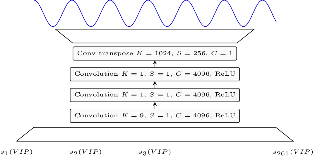
Takes the time representation at $62$ Hz and turn it into a waveform at $16$ kHz.
First convolution for temporal context. In place convolution for expressivity and final transposed convolution with large stride ($256$) for upsampling.
Spectral loss: the best of both world
SING generates directly the waveform.
Spectrogram is then computed using a differentiable implementation of STFT and the L1 loss is computed over log-power spectrograms.
Gradients are automatically computed.
No inversion problem but allows to use any differentiable signal processing transform (wavelet transform, mel-spectrogram etc).
Training
Take mirror image of the learnt upsampling as an encoder to form an autoencoder. Train for $12$ hours on $4$ GPUs.
Train the LSTM to match the output of the encoder using MSE and truncated backpropagation with length $32$ for $10$ hours.
Plug the decoder and LSTM and fine-tune end-to-end for $8$ hours.
In total $30$ hours on $4$ GPUs.
Plan for today
Experimental results
Reconstruction loss (reminder)
We want to evaluate the distance between the generated waveform $\hat{x}$ and the ground truth $x$. Either MSE on the waveform: \[ \newcommand{\abs}[1]{\left|#1\right|} \newcommand{\norm}[1]{\left\|#1\right\|} \newcommand{\Lwav}[1]{\mathrm{L}_{\mathrm{wav}}\left(#1\right)} \newcommand{\Lspec}[1]{\mathrm{L}_{\mathrm{stft,1}}\left(#1\right)} \newcommand{\STFT}[1]{\mathrm{STFT}\left[#1\right]} \newcommand{\reel}{\mathbb{R}} \Lwav{x, \hat{x}} := \norm{x - \hat{x}}^2, \]
or using a spectral loss: \[ \Lspec{x, \hat{x}} := \norm{l(x) - l(\hat{x})}_1 \] where $ l(x) := \log\left(1 + \abs{\STFT{x}}^2\right)$.
Ablation study
For unseen pairs of instruments and pitches, the MSE on the waveform and L1 on log power spectrograms are measured.
| Spectral loss | Wav MSE | ||||
|---|---|---|---|---|---|
| Model | Training loss | train | test | train | test |
| Autoencoder | wavform | 0.026 | 0.028 | 0.0002 | 0.0003 |
| SING | wavform | 0.075 | 0.084 | 0.006 | 0.039 |
| autoencoder | spectral | 0.028 | 0.032 | - | - |
| SING | spectral | 0.039 | 0.051 | - | - |
| SING no time embedding |
spectral | 0.050 | 0.063 | - | - |
With autoencoder, MSE on the waveform works well, model has access to input phase.
SING is purely generative. Has to remember by heart the specific phases of each note except when using a spectral loss.
Using a time embedding significantly improves accuracy.
Comparison with a Wavenet based autoencoder
Along with the NSynth dataset, Magenta released a Wavenet-based autoencoder.

Encoder has a Wavenet inspired architecture. Gives a vector of dimension $16$ every $50$ ms (compression factor $32$).
Decoder is conditioned on the temporal embedding.
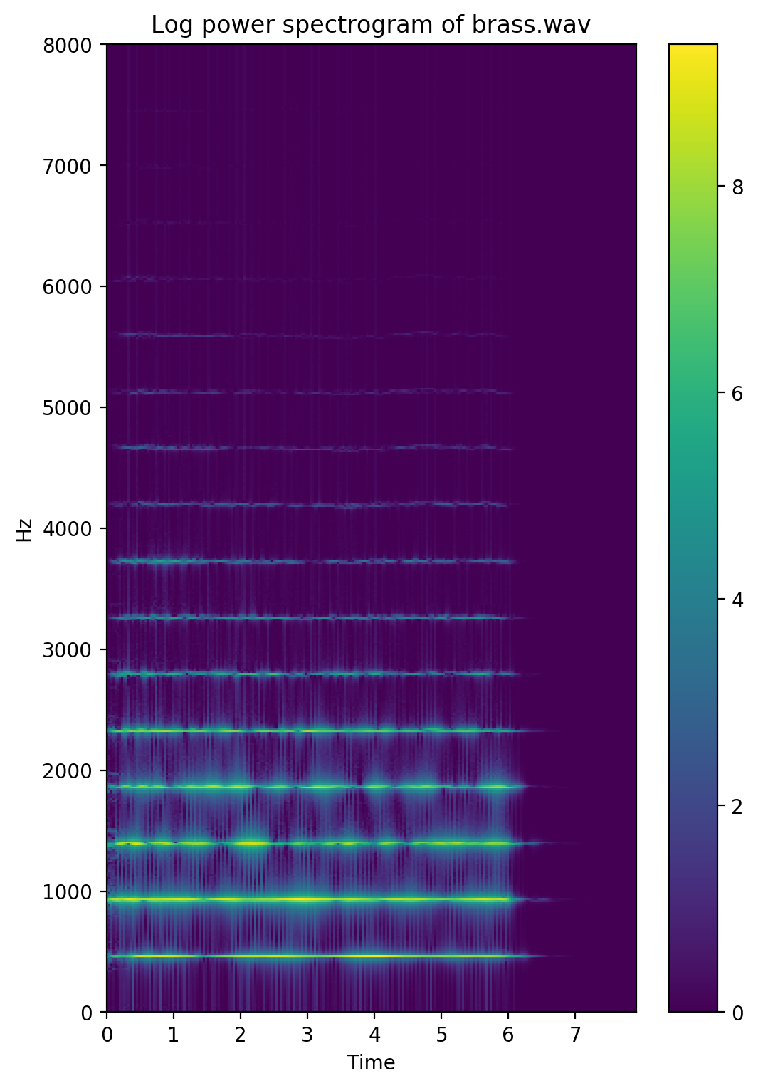
Quick audio comparison
| Instrument | Ground truth | Model A | Model B |
|---|---|---|---|
| Brass acoustic 001-054-127 |
|||
| Flute acoustic 027-077-050 |
|||
| Guitar acoustic 009-069-100 |
|||
| Vocal acoustic 023-057-127 |
Model A is SING and B is the Wavenet based autoencoder.
A more scientific human evaluation
MOS: for each model, 100 samples are evaluated by 60 humans on a scale from 1 ("Very annoying and objectionable distortion") to 5 ("Imperceptible distortion") using Crowdmos toolkit [paper] for removing outliers.
ABX: Ask 10 humans to evaluate for a 100 examples if Wavenet or SING is closest to ground truth. 69.7% are in favor of SING over Wavenet
| Model | MOS | Training time (hrs * GPUs) | Generation speed | Compression factor | Model size |
|---|---|---|---|---|---|
| Ground Truth | 3.86 ± 0.24 | - | - | - | - |
| Wavenet | 2.85 ± 0.24 | 3840 | 0.2 sec/sec | 32 | 948 MB |
| SING | 3.55 ± 0.23 | 120 | 512 sec/sec | 2133 | 243 MB |
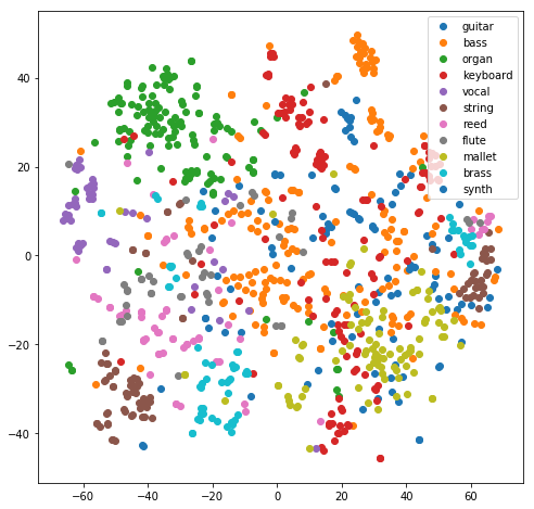
Instruments embeddings
Representation of instrument embeddings using T-SNE, colored by instrument family.
Plan for today
Conclusion and closing remarks
Conclusion
We have introduced SING, a lightweight and state of the art music notes generator as measured by human evaluations.
Thanks to its large stride rather than sample by sample approach, SING is trained $32$ faster than a Wavenet autoencoder and generates audio $2,500$ times faster.
A key novelty is being able to use an end-to-end spectral loss without having to solve the phase recovery problem explicitely.